Setting up a Control System
The control system shown in the diagram below monitors the temperature and if it is too hot it switches on a fan. If it becomes too cold it switches on a heater. For the purposes of keeping this simple a torch bulb will be used to represent the heater.
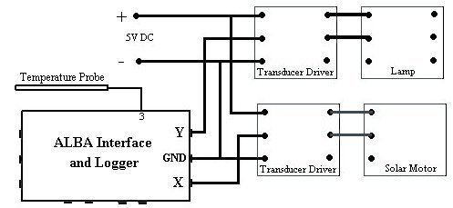
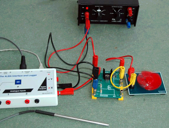
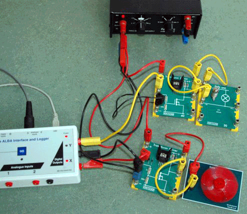
The test circuit used Unilab alpha boards for the Transducer Driver and Lamp. The djb Solar Motor represented the fan.
The photographs below show the fan under control then both the fan and lamp being controlled.
The Investigator software is used to control the outputs of the ALBA Interface and Logger.
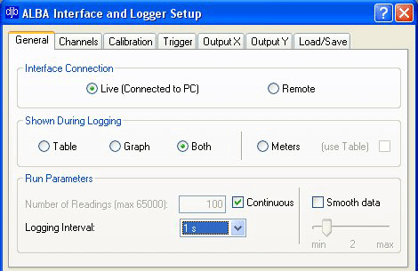 Step 1: Select the General Tab then enter suitable logging settings. Step 1: Select the General Tab then enter suitable logging settings.
Step2: Click on the Channels Tab and check that the software knows that a temperature probe is connected on channel 3.
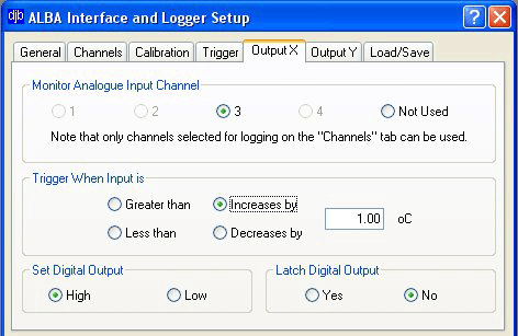 Step 3: Click on the Output X Tab. This example setup shows that channel 3 is being used for control and if the temperature ever increases by 1 degree then output X controlling the fan should be switched on. Note that you can control the output level of X ie when a target value is reached the output can be set to be high or low. Outputs may also be latched. Step 3: Click on the Output X Tab. This example setup shows that channel 3 is being used for control and if the temperature ever increases by 1 degree then output X controlling the fan should be switched on. Note that you can control the output level of X ie when a target value is reached the output can be set to be high or low. Outputs may also be latched.
A high on Output X corresponds to approximately 5V and a low to zero volts.
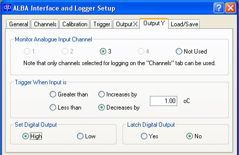 Step 4: Set up Output Y in a similar fashion. Step 4: Set up Output Y in a similar fashion.
It is worth noting that the analogue capture can have a digital trigger. This trigger could come from alpha boards eg when a person cuts a light beam the data capture starts. Science clubs could have some fun with this! |

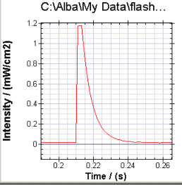 Connect the Linear light sensor to ALBA and set up the Investigator to take 1000 readings at 1ms intervals. No trigger was used but this could be investigated if desired. When you obtain the graph zoom in on the relevant portion.
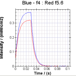 Set the 12V bulb supplied with the Inverse Square Law Kit immediately infront of the lens of an old fashioned SLR camera. Open the camera and place the Linear Light Sensor pointing through the lens. Set the speed to 1/30s and the f stop to f5.6.
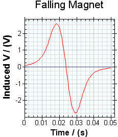 To obtain the results of a magnet falling through a coil as shown in the ALBA Software section of the site try the following:
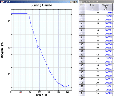 For this teacher demonstration you will require:
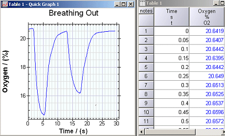 Connect your oxygen gas sensor to the ALBA Interface.